summarizeByVisitSCI() is the counterpart of
summarizeSCI() for data collected over several visits. It
produces the table of summaryByVisit() and one plot per
variable over the visits: a line plot (or boxplots) for continuous
variables and stacked barplots for categorical ones.
Table and plots
The arguments are those of summaryByVisit(). The visits
appear in the order of the table; with order, its values
also set the spacing of the visits in the line plot.
res <- summarizeByVisitSCI(hb, vars = c("hb", "hb_cat"), group = "Arm",
                           visit = "visit", order = "visit_nr",
                           stat_cont = "median_IQR",
                           labels = list(hb_cat = "Hemoglobin category"),
                           plot_args = list(risk_table = TRUE,
                                            group_names_short = c("A", "B")))
res$table
Visit |
N1 |
Arm A |
N1 |
Arm B |
|---|---|---|---|---|
Hemoglobin |
||||
Cycle 1 |
29 |
130.0 (127.0, 138.0) |
23 |
132.0 (120.0, 139.0) |
Cycle 2 |
83 |
135.0 (127.0, 140.0) |
84 |
133.0 (122.5, 139.0) |
Cycle 3 |
83 |
136.0 (129.0, 143.0) |
80 |
131.5 (124.0, 141.5) |
Cycle 4 |
80 |
136.0 (128.5, 141.0) |
73 |
133.0 (124.0, 138.0) |
Cycle 5 |
71 |
137.0 (128.0, 142.0) |
65 |
131.0 (124.0, 138.0) |
Cycle 6 |
69 |
137.0 (131.0, 143.0) |
62 |
131.0 (124.0, 137.0) |
Cycle 7 |
65 |
137.0 (129.0, 142.0) |
62 |
130.0 (123.0, 138.0) |
Cycle 8 |
60 |
136.0 (131.5, 141.5) |
62 |
130.0 (124.0, 139.0) |
Cycle 9 |
62 |
136.5 (130.0, 140.0) |
60 |
131.0 (124.0, 136.5) |
Hemoglobin category |
||||
Cycle 1 |
29 |
23 |
||
< 120 |
5 (6%) |
7 (8%) |
||
120-140 |
18 (21%) |
12 (14%) |
||
> 140 |
6 (7%) |
4 (5%) |
||
Missing |
55 (65%) |
62 (73%) |
||
Cycle 2 |
83 |
84 |
||
< 120 |
8 (10%) |
18 (21%) |
||
120-140 |
55 (66%) |
49 (58%) |
||
> 140 |
20 (24%) |
17 (20%) |
||
Missing |
0 (0%) |
1 (1%) |
||
Cycle 3 |
83 |
80 |
||
< 120 |
6 (7%) |
12 (15%) |
||
120-140 |
49 (59%) |
47 (57%) |
||
> 140 |
28 (34%) |
21 (26%) |
||
Missing |
0 (0%) |
2 (2%) |
||
Cycle 4 |
80 |
73 |
||
< 120 |
8 (10%) |
15 (20%) |
||
120-140 |
49 (61%) |
46 (62%) |
||
> 140 |
23 (29%) |
12 (16%) |
||
Missing |
0 (0%) |
1 (1%) |
||
Cycle 5 |
71 |
65 |
||
< 120 |
5 (7%) |
9 (13%) |
||
120-140 |
43 (59%) |
45 (67%) |
||
> 140 |
23 (32%) |
11 (16%) |
||
Missing |
2 (3%) |
2 (3%) |
||
Cycle 6 |
69 |
62 |
||
< 120 |
2 (3%) |
9 (14%) |
||
120-140 |
42 (61%) |
46 (71%) |
||
> 140 |
25 (36%) |
7 (11%) |
||
Missing |
0 (0%) |
3 (5%) |
||
Cycle 7 |
65 |
62 |
||
< 120 |
5 (8%) |
7 (11%) |
||
120-140 |
37 (57%) |
44 (70%) |
||
> 140 |
23 (35%) |
11 (17%) |
||
Missing |
0 (0%) |
1 (2%) |
||
Cycle 8 |
60 |
62 |
||
< 120 |
4 (6%) |
9 (15%) |
||
120-140 |
38 (59%) |
42 (68%) |
||
> 140 |
18 (28%) |
11 (18%) |
||
Missing |
4 (6%) |
0 (0%) |
||
Cycle 9 |
62 |
60 |
||
< 120 |
3 (5%) |
7 (12%) |
||
120-140 |
44 (70%) |
46 (77%) |
||
> 140 |
15 (24%) |
7 (12%) |
||
Missing |
1 (2%) |
0 (0%) |
||
1N without missing values | ||||
2Median (Q1, Q3); n (%) | ||||
res$plots$hb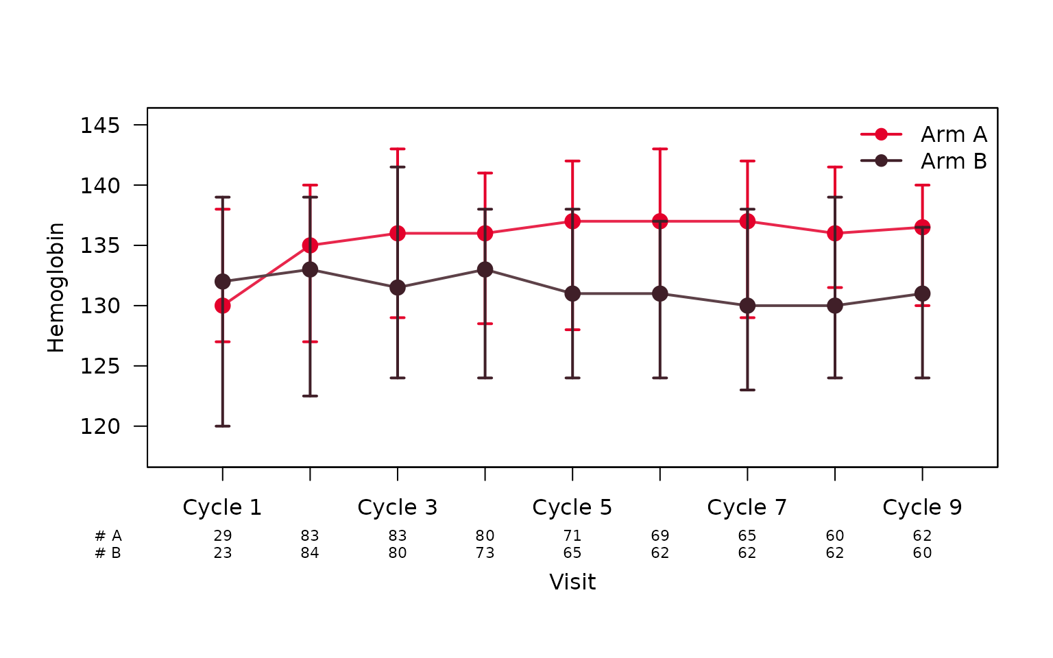
res$plots$hb_cat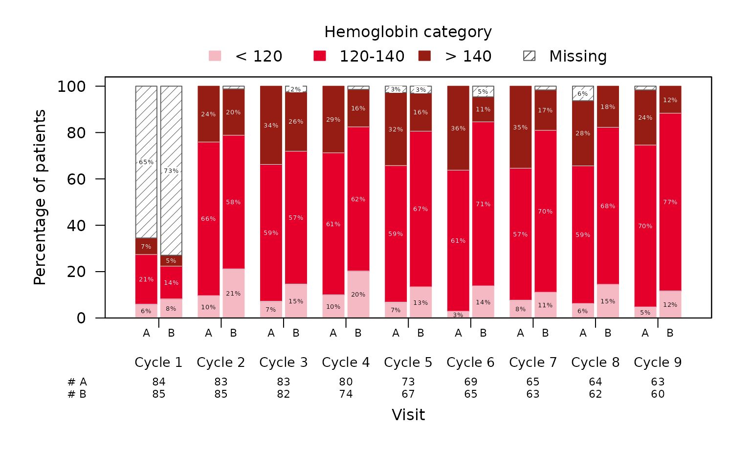
As in summarizeSCI(), type = "table" or
"plot" returns only one of them, the table’s settings
(labels, missing, missing_percent,
stat_cat) carry over to the plots, and further plot options
go into plot_args (see ?lineplotSCI,
?boxplotSCI and ?stackedbarplotSCI).
The plots show the numbers of the table
The line plots and stacked bars are drawn from the numbers printed in
the table, as plotByVisit() does: they show exactly what
the table shows, with its rounding, its visits and its N columns as the
risk table. stat_cont decides what the line plot shows:
stat_cont |
Point | Error bars |
|---|---|---|
"median_range" |
median | minimum to maximum |
"median_IQR" |
median | first to third quartile |
"mean_sd" |
mean | +/- one standard deviation |
"mean_se" |
mean | +/- one standard error |
"geomMean_sd" |
geometric mean | ÷ and × geometric SD |
The geometric mean needs positive values: the table shows
NA for visits with values of zero or below, and the line
plot leaves those points out.
plot_args = list(stat_footnote = TRUE) names the statistic
in a footnote under each plot.
plot_cont = "boxplot" draws boxplots per visit instead
of the line plot. A boxplot shows more than the table holds, so it is
drawn from the data: from the rows the table summarizes, with the box at
the quartiles as the table computes them. It always shows the median and
quartiles, whatever stat_cont the table uses; with
"median_IQR" the two agree.
res_box <- summarizeByVisitSCI(hb, vars = "hb", group = "Arm",
                               visit = "visit", order = "visit_nr",
                               stat_cont = "mean_sd", plot_cont = "boxplot",
                               plot_args = list(cex_axis = 0.8))
res_box$plots$hb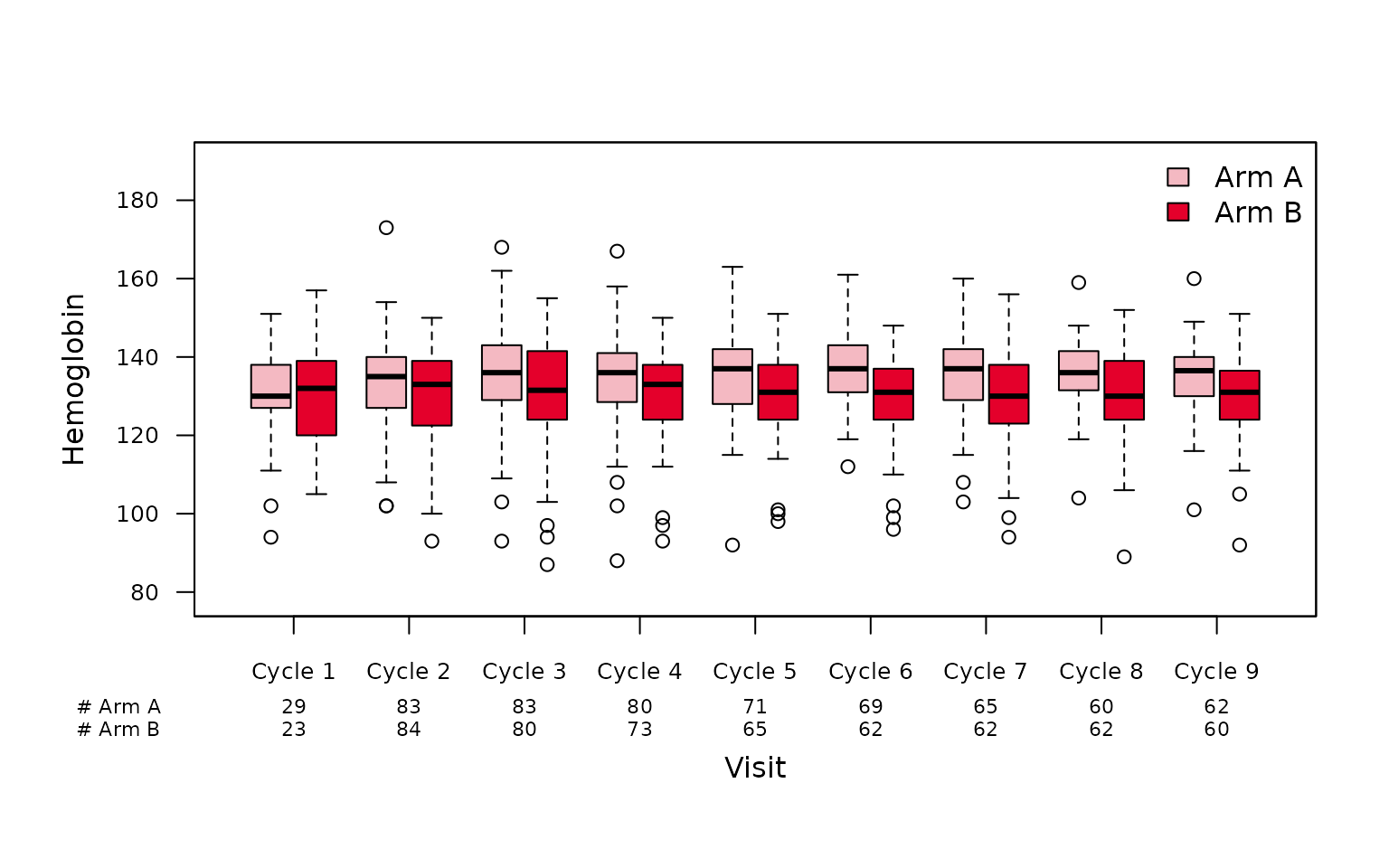
Saving the table and plots
word_output = TRUE (with file_path) and
save_plots() work as described in
vignette("summarizeSCI"):
basename(save_plots(res, file_name = "visit", file_path = tempdir(),
                    width = 9, height = 5.5))
#> [1] "visit_hb.png"     "visit_hb_cat.png"