Plot a summaryByVisit table

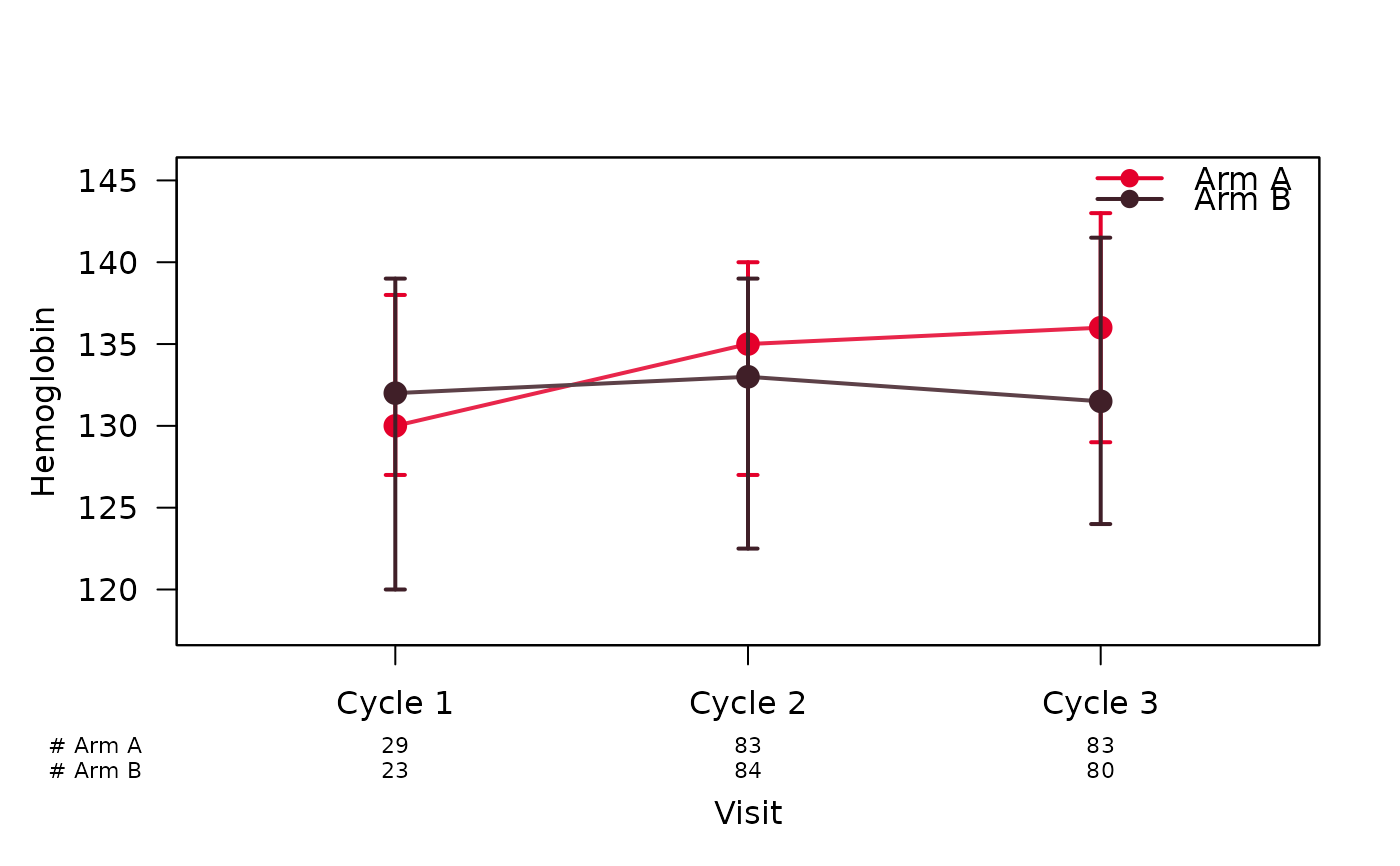
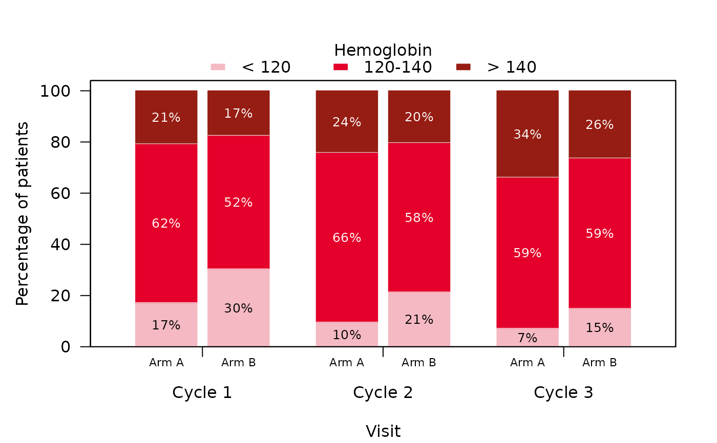
Plots one variable of a table produced by summaryByVisit() over the visits, using the numbers printed in the table rather than the raw data. Continuous variables are drawn as a line plot of the point estimate with its interval (see lineplotSCI()), categorical variables as stacked bars (see stackedbarplotSCI()).

Usage

plotByVisit(
  tbl,
  var = NULL,
  stat_cont = NULL,
  missing = FALSE,
  missing_text = "Missing",
  ...
)

Arguments

tbl

A table returned by summaryByVisit() with as_flex_table = FALSE (the default TRUE returns a flextable, from which the numbers cannot be read back).

var

The variable to be plotted, given as its label in the table (the bold header row, e.g. "Hemoglobin") or its position among the variables of the table. May be omitted if the table holds a single variable.

stat_cont

The statistic of continuous variables, as passed to summaryByVisit(). Default is NULL, which reads it from the table footnote; if the footnote is not recognised, plotByVisit() stops and asks for stat_cont rather than guess. A stat_cont that does not fit the printed cells (e.g. "mean_sd" for a median (range) table) is an error too.

missing

A logical toggle switch adding the missing-value rows of a categorical variable as a segment of their own. Default is FALSE, which leaves them out, so that percentages are relative to the non-missing observations.

missing_text

The label of the missing-value rows in the table, as passed to summaryByVisit(). Default is "Missing".

...

Further arguments controlling the appearance of the plot, as documented in lineplotSCI() (continuous variables; e.g. interval_type, risk_table, col, legend_position) or stackedbarplotSCI() (categorical variables; e.g. scale, percent_labels, risk_table). For continuous variables, xs sets the positions of the visits on the x-axis (one number per visit, e.g. the study days); by default they are evenly spaced.

Value

Invisibly, a list with

• type: "continuous" or "categorical";

• summary: the rows of tidySummaryByVisit() belonging to var;

• for continuous variables, the group-by-visit matrices centre, lower, upper and n;

• for categorical variables, the arrays counts and percent indexed by level, group and visit, and the group-by-visit matrix n of denominators.

Details

The statistic of continuous variables is read from the table footnote and determines the error bars:

• "median_range": median with whiskers from minimum to maximum;

• "median_IQR": median with whiskers from the first to the third quartile;

• "mean_sd" / "mean_se": mean +/- one standard deviation / standard error;

• "geomMean_sd": geometric mean divided and multiplied by the geometric standard deviation.

Since the numbers are read from the printed table, they carry its rounding (digits_cont / digits_cat). Visits appear on the x-axis in the order of the table rows.

Examples

library(summarySCI)
data("hemoglobin_data")
hb <- subset(hemoglobin_data, visit_nr <= 3)   # first 3 cycles, to keep it short
attr(hb$hb, "label") <- "Hemoglobin"           # subset() drops the label
tbl <- summaryByVisit(hb, vars = "hb",
                      group = "Arm", visit = "visit", stat_cont = "median_IQR",
                      as_flex_table = FALSE)
plotByVisit(tbl, var = "Hemoglobin", risk_table = TRUE)


# \donttest{
# a categorical variable
hb$hb_cat <- cut(hb$hb, c(-Inf, 120, 140, Inf),
                 labels = c("< 120", "120-140", "> 140"))
tbl <- summaryByVisit(hb, vars = c("hb", "hb_cat"),
                      group = "Arm", visit = "visit", stat_cont = "median_IQR",
                      as_flex_table = FALSE)
plotByVisit(tbl, var = "hb_cat", legend_title = "Hemoglobin")

# }